Home Science Page Data Stream Momentum Directionals Root Beings The Experiment
Let us try another approach to Decay and Sensitivity. The first we will describe is the Short Term Average. This style of average behaves like a short-term memory system. The most recent input replaces the oldest input. There are not that many pieces of Data. The Data comes in quickly and goes out quickly. This average immediately throws away the past, replacing it with the present. I will restrain myself from finding anything analogous in Pop culture.
The Traditional Average, the Mean, weighted all data, past and present, equally. While taking all the Data from the Stream into account, this measure lacks sensitivity to the Ordered nature of Data Streams. While the Short Term Average weights the most recent data more heavily, it immediately 'forgets' the past, replacing it with the present. We need an average, which takes the past into account while weighting data by its proximity to the present. Enter the Decaying Average. With the Decaying Average, each bit of Data enters the Data Stream and immediately begins decaying. The past is discounted but not entirely 'forgotten', as with the Short Term Average. Before going on let us discover the Decaying Average. Then we will examine its implications.
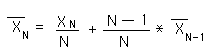
In the Notebook, 'Data Stream Momentum', we derived the following context-based equation for the mean of a Data Stream.
This equation allowed us to compute each subsequent mean in the Data Stream without having to 'remember' all of the previous pieces of Data in the Stream. In this style of computation each average is generated from the previous average and is itself the source of the next average. Only three elements are needed to compute the new average, the new data point, the old average and the number of elements in the stream. Because the new data point is 'experienced' only two elements need to be 'remembered', i.e. the previous average and N, the number of elements. The 'problem' with this equation in describing a Data Stream sensitively is that the potential impact of each successive piece of data is diminished, because N continues to grow. We would prefer that it remain the same.
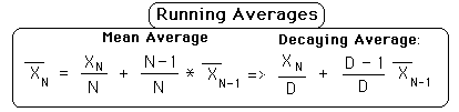
To simplify our 'memory' and to achieve our ends let us fix N.
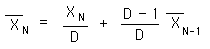
This is the defining equation for the Decaying Average. Because we are fixing N at a predetermined value, it will no longer reflect the number of samples. We will no longer call it, 'N', the Number of samples. We will now call it, 'D', the Decay factor. Now each New Data Bit has the same potential for Impact because D, is not growing with each new data bit, but remains the same.
Notice that the new average is determined by the old average, the new Data Bit and D, the Decay Factor. While the computation of the Mean Average of our Data Stream required the 'memory' of two bits of data, the Decaying Average only requires the 'memory' one piece of data because D is a preset constant, not a growing sample number. Thus the Decaying Average, not only equalizes the potential impact of each successive piece of data, but is also simpler to compute, needing only one data bit.
Let us now look at the definitional equations of the 3 averages we have discussed so far. The Mean Average has two definitional equations. They are equivalent but lead in different directions.
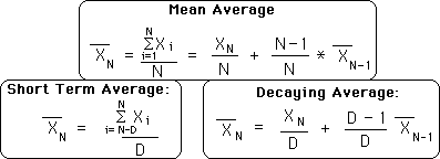
Notice how the Short Term Average is derived from the first definition of the Mean Average while the Decaying Average is derived from the second definition of the Mean Average.
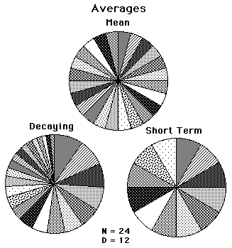
The following pie graphs show the composition of each of the 3 types of averages that we've discussed. Each piece of pie represents the potential impact of that piece of data in that type of average. The gray piece between 12 Noon and 1PM is the last piece of the Data Stream. Clockwise around the circle are the next to last, and so forth, until we reach the most distant data Piece that still has an impact upon the average. The Short Term Average goes back only 12 Data Pieces, while the Mean and Decaying Averages go back to the beginning of the Living Data Set. Notice how each of the pieces in the Mean Pie and the Short Term Pie are equal, while the Decaying Average Data Pieces are arranged from large to small from present to the past.
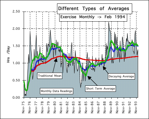
Notice in the graph that the gray area represents the Real Monthly Data. This is what we want our averages to reflect.
The Red Line represents the Traditional Average over all the data points. Notice as the set grows larger and larger the red line becomes more and more steady. While doing a good job of reflecting the whole set, its most recent readings, on the right, are totally out of touch with the changes that are going on. The Traditional Average is ponderous due to the growing size of N, the number of samples. It is rutted in the past, giving each point equal weight, regardless of proximity to the present.
The Green Line represents the Short Term Average where N = 12, i.e. the averages are calculated over just the last 12 data points. While much more in touch with the present it is out of touch with the past. The N = 12 Average is highly volatile. It is quick to throw away the past in honor of the present. It reflects the present more accurately because it has forgotten about the past. While sensitive to present changes, it has lost its sense of history.
The Blue Line represents the Decaying Average, when D = 12. It tends to reside between the Red and Green Line. With the Decaying Average, each bit comes in at its occurrence and then begins to decay. The past counts but is depreciated to give more emphasis to the present. The Decaying Average takes the past into account but gives more emphasis to the most recent Data Bits.
It has been discovered that computational ability is an evolutionary advantage just as is strength, speed, or size. Those creatures that can most accurately estimate distances will survive more frequently in a terrain with many cliffs. Mountain goats with a poor sense of distance estimation did not survive to pass on their gene pool.
In terms of evolution, the simpler computations also have an advantage over complex computations for two reasons. First, it is more likely to evolve taking small simple steps than making complex computational leaps. Second it is easier to pass on something simple, less likely for error. To evolve into taking derivatives of functions would take longer than to evolve into doing simple sums because of the complexity of the process.
The creature that can remember the past as well as being sensitive to the present will also have an evolutionary advantage. If a creature abandons the past in his sensitivity to the present, he may forget an ancient enemy and will not pass his gene pool on. Conversely a creature, who is so tuned to the past that he can't adapt to environmental changes, will also be at an evolutionary disadvantage. Man's ability to adapt to change was what enabled man to survive and thrive in a hostile environment, with many stronger and quicker creatures.
We have identified 3 evolutionary advantages: 1. the ability to compute, 2. simple computations, 3. sensitivity to past and present. Which of our three central tendencies rates highest in terms of evolutionary fitness? Which average measure would most enhance a creature's fitness for survival?
In terms of sensitivity to the past and the present, Decaying Averages certainly wins out. The Short Term Average throws away the past in its sensitivity to the present. It is too volatile. The Traditional Average is sensitive to neither past nor present in its desire to treat each Data Bit equally. It is too cumbersome. The Decaying Average diminishes the past but does not throw it away. The present is emphasized, but the past remains.
But, you, the Reader say, how can anything but a complex computer program compute a Decaying Average that doesn't forget the past, and diminishes each data point according to its size and proximity to the present. It would seem that an incredible amount of memory would be needed to store all that information. You, the Reader, think to yourself, the Decaying Average certainly reflects the past and present more accurately than the others but will certainly lose when it comes to the simplicity of the computation. Read on for the surprising results.
Let us rate the complexity of calculations by three factors: 1. the complexity of the operation, 2. the number of facts stored, 3. the relevance of the facts. The complexity of the operation used to generate the results is of crucial importance. In terms of operations, one hyperbolic cosine operation would sink the Simplicity ship, as would most of the trigonometric functions. Humans do well with adding, subtracting, multiplying and dividing, while more complex operations are usually reserved for computers. Evolving to do summations and divisions is simple vs. the more sophisticated operations.
The second factor is the number of facts that need to be stored to perform the calculation. If the organism needs to store a dozen facts to make the next computation, he has a greater chance for error than does an organism that only needs to store two facts. The less the number of facts that need to be stored the better.
The third factor is the more relevant the fact is the easier it is to store. Evolutionarily we only store facts with relevance. Storing a number with no inherent meaning is less likely than storing a number with lots of inherent information.
With these three factors in mind, let us look at the three types of averages that we are considering. To calculate a Short Term Average, the organism needs to store a sequence of data, ordered bits of information. Then it must perform an addition, a subtraction, and a division. Seeing as how memorizing a seven digit phone number is an act of will for most people, we will consider storing a sequence of semi-relevant ordered data as an excruciating and thereby unlikely evolutionary event for long term events. This type of average would come in extremely handy on a short term immediate level, perhaps combat, where old data needs to be immediately thrown away to be replaced by the new data, as to position, velocity, and acceleration. This type of average acts like the short-term memory. The newest bit squeezes the oldest bit off the end of the bench. This type of average would never be able to analyze long-term trends or tendencies.
The first definition of the Mean Average is only for calculators. The organism would either have to store every data bit that entered under its category, or it would have to store the accumulation and the number of data bits. If a short sequence of ordered data bits is difficult and only useful in short term memory, then storing an ever-increasing number of data bits is even more unlikely. Also the storage of an accumulated number that is continually growing is equally unlikely for two reasons. One, this sum of a growing number of data bits has no relevance to anything. Two because of its lack of relevance, except for calculation, it is highly prone to error. If the sum or the number of data bits were distorted in any way then the Mean would be thrown way off. The Mean Average of a Living Set could only be computed with a calculator, not by evolutionary organisms; there is not enough relevance. This Average could have relevance for the long-term perspective, but could only be approximated not calculated.
For the primitive organism, summations are out. They are cumulative with a sum, which has no reference to reality, and a cumulative number of trials, which also bears no reference to reality. So the first definition of Mean Average is out. The Short Term Average has the advantage that it deliberately limits the number of Data Choices to the most recent events. Therein lies its usefulness, but it throws away the Past.
The second definition of the Mean Average is far superior to the first in that there are no summations. Retaining the exact number of trials, N, would be difficult, as in the first definition. However retaining the past average, a running average, is something that could be quite useful for prediction. We'll talk about this later.
We've shown that the Decaying Average is not as volatile as the Short Term Average. It is also more responsive than the Traditional Average, the Mean. Now it will be shown that the Decaying Average is also the easiest to calculate because it involves no summations and stores the highly relevant Running Average. The Decaying Average evolves from the second definition of the Mean Average. It retains the running average that is a relevant piece of data because of its power for prediction. It, also, transcends the problem of accumulating N, the number of trials. D, the Decay Factor, is a flexible constant that is determined by experience.
The Decaying Average makes use of the way that the Mean Average is formed. 1. Take the latest piece of data, the freshest. Put it on top of the old average. If it is smaller, then subtract a little from the old average; if it is larger then add a little to the old average; if it is the same then leave it alone. 2. Take the next piece of data and repeat the same process. The process could be repeated indefinitely, generating a deeper and deeper average because the repetitions leave a deeper and deeper impression on the neural networks. The center of the average is strong but the edges are fuzzy because they leave trace lines of the averages that went before. The total number of samples has no bearing upon the generation of a running average. Just add a little, subtract a little.
How much is to added or subtracted each trial? The Mean Average would adjust less and less proportionately as time went on. After only a 100 repetitions the influence, the potential impact, of the new Data Piece would be almost negligible upon the Running Average. For the Decaying Average the potential impact of each new Data Piece would be equal, if D, the Decay Factor, is consistent.
How is D, the Decay Factor set? This is a matter of experience. The Running Average is a predictive measurement. If D is set low then history is minimized. If D is set high then history is maximized. So each phenomenon with its own unique Data Stream is evaluated accordingly. With some Data Streams, history is unimportant. When D is set at 1, the past loses all relevance. This describes dynamic systems, which are predictive. Give an initial point and all else is predictable. Past and future are unimportant. When D is set higher, the adjustments to the Running Average become proportionately smaller. The past is given more weight and the present is given less weight as D increases.
The purpose of the accumulation of the running average is to assist in anticipation. If the prediction of the active organism is wrong, then the next prediction is moderated accordingly. The purpose of prediction is anticipation and anticipation aids survival. Those whose predictions are most successful are the most likely to survive and propagate. Therefore the ability to calculate the running average was an early and easy evolutionary advantage, coming alongside and within the neural network.
In some ways, neural networks were set up to calculate Running Averages, which are a type of Decaying Averages, where D is a semi-consciously adjusted variable based upon experience. The organisms whose D's are most accurate is most likely to anticipate and survive. When D is constantly increased to equal the number of samples, the Running Average would equal the Mean Average. When D is kept fixed then the Running Average is a pure Decaying Average. In real life D, the Decay Factor, is constantly changed based upon the accuracy of predictions. In our studies, we will keep D fixed for consistency.
The early homo sapiens sapiens were able to survive because they were able to anticipate seasons. Those who planted off-season would have a poorer yield. Those who didn't anticipate winter didn't have enough to survive. Seasonal anticipation was based upon one of the first long-term predictions, the annual prediction. The Sun has retreated as far as it is going to go and will now return. In most cultures, the prediction of Winter & Summer Solstices has been crucial to the survival of the tribe because it helped them to anticipate seasonal changes.
Because the Decay Factor is flexible, it varies from person to person, age to age, philosophy to philosophy. Following is a brief discussion of different modern interpretations of the Decay Factor, intentional and unintentional.
Popular culture tends to change its Decay factor regularly. Their D is so unstable that it bends with the media wind. Scientists, on the other hand, tend to stick to a Decay Factor of 1. They try to reduce any phenomenon to a condition where D = 1. In fact the one reason that Physicists are so proud historically is that they have been able to reduce so many phenomenon to a condition where D = 1. If a physicist dies without being able to turn a phenomenon into a D = 1, he is considered a failure, will not be given tenure, will be forgotten and unpublished. D=1 describes any phenomenon which can be reduced to a precise linear equation. {See Live & Dead Data Set Notebook.}
The Decay Factor, as we shall see in the Boredom Principle Notebook, is almost a factor of personality. Those with a low D tend to become bored more quickly. The Taoist approach would be to be consistently aware of a range of Decay Factors, rather to be fixed on one, many or none. Many Eastern religions focus upon none. Lose attachment to this plane. With their experimental the Taoists approach is trying to grab the Ungrabbable, explain the Unexplainable. We are forever making predictions and testing results. But we try to be unattached to our own hypothesis.