Home Science Page Data Stream Momentum Directionals Root Beings The Experiment
We’ve found an F&D Series for both square roots and cube roots. There are similarities and differences between the two sets of F&D Series that are intriguing. Naturally, through the mechanism of curiosity, we will now explore the F&D Series for the fourth root.
For ease of expression, the rational number that we are attempting to find the fourth root of we will refer to as the Root Number, or simply Number, if the context calls for it. Similarly we will refer to the actual fourth root as the Root. Either of these references can be general or specific depending also upon context. If there is a need to be more specific then a number will be appended to the end. As an example Root3 of Number3 would mean the cube root of some rational number.
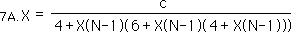
Let us begin the same way we did when exploring square and cube roots. We assume that X+1 equals the fourth root of some rational number. We raise each side to the fourth power. We subtract one from both sides of the equation. We factor out an X from the left side of the equation. We introduce ‘c’ as a constant, which is a function of ‘a’ and ‘b’, the elements of our rational number, a/b. We then divide both sides of the equation by the other factor on the left. Finally we nest the X factors in a more useful fashion for the purposes of this study.
Equation 7 is an example of X as a function of itself. This type of equation can and is meant to be iterated. Like last time, if we iterate this equation, all at once, it works well with positive numbers under 10, but bifurcates with the larger numbers. It is a bogus F Series. It is shown below.
When ‘c’ is between +1 and -1, then the X of 7A approaches the same limit as the X of Equation 7 when iterated. However when c becomes too large the X of 7A bifurcates into two numbers that are not equal to the X of equation 7. This was discovered through computer testing.
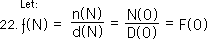
Last time we tried a different approach to iteration. Although it would be interesting to break down this fractal display, one step at a time like we did last time, there is a simpler way that we will exploit. First let us remember the X and ƒ functions that we developed in our discussion of cube roots. The X(N) functions were simply a method of expanding the original equation for X, i.e. equation 7. Our only rule was that we expand the leftward X first. By definition X(N) transforms into X(N+1) when it is expanded. This was all demonstrated amply in the algebra of the last section. Further we set up the ƒ fractions to approximate the X functions. While X(N) always equaled the Root-1 the ƒ(N) fractions only approximated it. However as N approached infinity, ƒ(N) also approached the Root-1. To obtain the values of the ƒ(N) Series, we treated each X in the corresponding X(N) Series as if it were equal to zero.
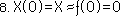
Let us demonstrate. X(0), the X that has been iterated zero times, is X itself. Therefore ƒ(0) the approximation equals zero, according to the rule that all Xs in the corresponding X series equals zero.
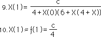
With the first iterated X, X(1), we get the first expression for X, the general equation 7. We introduced the X(0) just to cement the relations and equalities.
Letting X=0, according to the definition of the ƒ Series, we find that ƒ(1) = c/4.
The second iterated X, X(2), is the general equation X(1) with the leftward X expanded. According to the definition of expansion, X(0) becomes X(1). This is shown below.
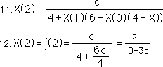
We are able to evaluate this expression for ƒ(2), an approximation of X(2), as X(0) or X is still equal to 0 while X(1) is equal to c/4. This is shown above. This is only the second iteration and it is already getting complicated.
In the third iteration, we follow the same rules of expansion of the X Series. X(1) becomes X(2); and the next X is iterated for the first time becoming X(1).
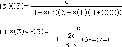
ƒ(3) can be easily evaluated using the values for ƒ(1) and ƒ(2), which are approximations of X(1) and X(2) respectively. This mess is shown above. It is obvious that the complexity is increasing.
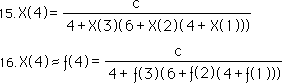
Using the same process we can easily obtain the expansion of X(3) into X(4). While X(4) equals the Root minus one, ƒ(4) is a practical approximation of this idealized value. This is shown in Equation 16.
While we could easily replace ƒ(3), ƒ(2), and ƒ(1) by the constants derived above, this would only lead to more complexity. Thus we will leave it in this more general algebraic expression, which is still easy to evaluate.
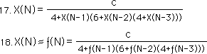
Employing the same style of generation, it is easy to see that as the X function is expanded that the elements in the denominators of equations 15 and 16 are also expanded by one. This leads to the general equation for X(N) listed below in equation 17.
Further the approximation of the X(N) function is ƒ(N), listed in Equation 18.
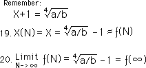
Let us return to the roots of this algebraic demonstration, remembering that we started out by ‘letting’ X+1 equal the fourth root of some rational number, a/b.
This means that the X(N) functions, all equal the Root minus one, which is approximated by ƒ(N). However as N approaches infinity, ƒ(N) approaches the Root minus one. We signify this as ƒ(∞). Thus X equals the limit of the ƒ function as it approaches infinity. Thus ƒ(N) approaches the Root minus one, the more it is iterated.
Now that we have discovered the ƒ Series for the 4th root, let us find the Denominator Series.
We begin, as before, by assuming that a Numerator and Denominator series exist. Further we show two parallel systems of notations.
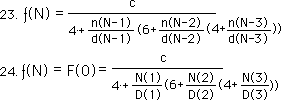
We substitute these expressions for the numerator and denominator series into Equation 18.
Equations 23 and 24 are equivalent. Equation 23 shows the iteration sequence more clearly, while Equation 24 is more concise. We will use the notation of Equation 24 for this reason.
We ‘simplify’ the equation by normal algebraic means. We combine denominators and then multiply top and bottom by the common denominator. Equation 25 is the result.
As before, we notice that the numerator is expressed solely in terms of the Denominator series.
Substituting this result for the Numerator series of equation 25, we obtain this result.
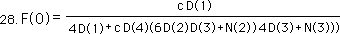
We factor out the D(2)D(3) from the denominator and then cancel out the common factor from the numerator, realizing that D(2)D(3) divided by itself is one, the identity property. (We’re trying to be a little more formal, as best we can.) This leaves us with the following reduced expression.
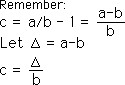
Remember the delta, ∆, terminology.
We convert the ‘c’ of equation 28 to the delta terminology in order to be more concise. This is equation 29.
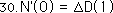
Once more we notice that the new numerator series, noted as N’(0) below, is a function of the previous denominator. This is expressed below.
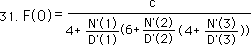
As before, under our discussion of cube roots, we assume that a Numerator and Denominator series for the 4th root exist with that relation. We substitute this N’ and D’ series into Equation 18 and obtain the following.
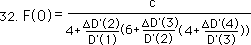
We then substitute the assumed relation of equation 30 into equation 31.
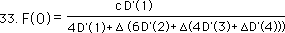
We combine terms with the common denominator of D’(3) in the most rightward expression in the denominator. The D’(3) denominator cancels out with the previous numerator. We then combine the middle terms with the denominator of D’(2). This then cancels out with the preceding numerator. Next we combine the left most terms in the denominator by combining with D’(1). Multiplying the top and bottom of the right side of the equation by D’(1), using the identity principle, we obtain the following equation.
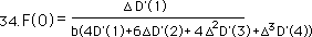
Converting to the ∆ notation, we obtain the following.
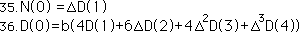
This proves our original assumption that a Numerator series exists where N’(0) equals ∆D’(1). Simultaneously it shows us what this Denominator series is. These two relations are shown below.
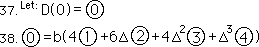
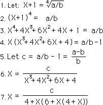
The D series for the 4th root are shown with the circle notation, defined below.
Remembering the subscript notation developed previously, the Denominator series for the fourth root should have a subscript of 4.
Now we can state our three basic iterative Theorems for Fourth Roots. These are the F Series Theorem, the Numerator Theorem and the Denominator Theorem, i.e. the First, Second and Third Theorems in that order. While these Theorems have not been thoroughly established deductively, they have been tested under a variety of circumstances always yielding the fourth roots of the appropriate numbers. The likelihood of ‘accidentally’ coming up with the fourth root of any number is so unlikely that we are safe in saying that these Theorems for fourth roots have been conclusively verified experimentally.
Let us begin with the First Theorem, the F Series for fourth roots.
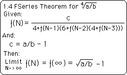
This theorem states the third order iterative expression, i.e. three layers of feedback, which the F Series for fourth roots is based upon. It then points out that the Limit of this iteration, i.e. as the number of iterations approaches infinity, is the Fourth Root of our rational number, a/b, minus one.
Note that we number this First Iterative Theorem for fourth roots as '1.4'. The '1' signifies that it is the F Series Theorem. The '.4' signifies that it is for fourth roots. Similarly we should have called the F Series Theorems for square roots as 1.2 and the F Series Theorem for cube roots as 1.3. With a deeper understanding that we will develop a little later on these delineations become somewhat unnecessary.
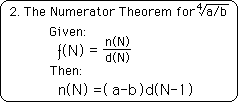
The Second Iterative Theorem for fourth roots, the Numerator Theorem is shown below. It is identical to the Numerator Theorem for cube and square roots. For this reason, it is just called the 2nd Theorem rather than the 2.4 Theorem, which is equal to the 2.3 and 2.2 Theorems.
The Third Iterative Theorem has to do with the relation between the F & D Series. It is called the Denominator Theorem. The Third Theorem for fourth roots is shown below. Because the D Series is different for the 2nd, 3rd and 4th roots, we call this the 3.4 Theorem to signify that it refers to fourth roots.
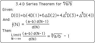
Note that while the iterative expressions for the D Series is different for fourth, cube and square roots that the relation of the D Series to the F Series is identical.