Home Science Page Data Stream Momentum Directionals Root Beings The Experiment
Remember our expression, ‘Wherever there are the coefficients of Pascal’s triangle, there is a binomial expansion, not far behind.’ This section is devoted to the Binomialization of the F&D Series.
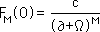
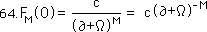
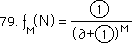
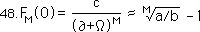
Let us begin with the end for a change. Below is the general binomialized expression for the F Series for the Mth Root of any rational number, a/b, where c=(a-b)/b, as normal. M is a positive integer. (This treatment also applies to fractional roots. The constant c would simply equal the general expression for c listed above. We just chose integer roots for simplicity of expression.)
Now all we need to know is what ∂ and Ω, represent. This is the shocker.
The first element, ∂, represents an infinitesimal, while the second element, Ω, represents a dimensional generator. For short we will call Ω a generator. Neither is a normal number. While the elements of the Denominator and Fraction series are all regular numbers, these are not. Because ∂ and Ω are not and do not represent regular numbers, they also do not combine the same way as regular numbers do. Hence the operations of the binomial expansion need to be defined.
Following are some of the questions that need to be answered. What happens when an infinitesimal is added or multiplied times a generator? What happens when an infinitesimal or generator is added or multiplied by itself? The question we don't need to know, and can’t answer, is why it happens.
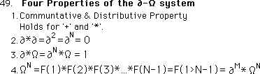
Infinitesimals are so small that when added or multiplied by themselves they always equal an infinitesimal, which equals zero in our plane. However an infinitesimal is not equal to zero, they represent something. Hence when an infinitesimal is added or multiplied times a generator it equals something, in this case 1, unity, the all. Generators, on the other hand, only achieve ordinary reality when they are combined with something else. Generators multiplied by themselves raise the number of elements of the F series multiplied times each other. This is probably far too confusing to be understood independent of the numbers themselves. Listed below are the relations for the F Series.
Before exploring their manifestations let us look at the properties themselves to understand them. Property #1 is mandatory if the binomial expansion is to work. At first glance Properties 2 and 3 seem contradictory. However when it is realized that neither ∂ nor Ω are regular numbers, nor is ‘*’ a ‘regular’ multiplication, we can begin to make sense of it. First ∂ is an infinitesimal, a point; it is not really nothing. Thus whether it is a square point or whether it is cubic or quartic point, it is still an infinitesimal. Thus its size relative to anything is still zero, although it still exists. Thus when it is combined with Ω, it still equals something, i.e. one. Property 4 merely states that the exponent of Ω indicates how many of the F series are to be multiplied times each other. Soon we will see examples of this property.
Perhaps we should have stated that ∂ equals a different type of zero to make sense of these equations. Perhaps we should have said that ∂ raised to any power and added to something always equals that something. This alternative way of expressing the property is shown below.
This representation of property 2 doesn’t really equate ∂ with zero. But any standard algebraic manipulation would immediately prove that it equals zero. Thus we must stress verbally that it equals an infinitesimal, which exists, although it is infinitely small.
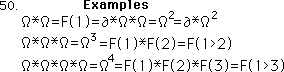
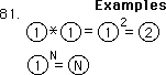
Here are a few examples of these properties in action.
Let us do a few simple expansions of our F Series to see what we’re talking about. This is the general equation for the F Series from equation 48.
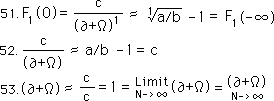
Let us start at the beginning when M = 1. Substituting in the general equation.
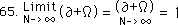
In step 51, it is remembered that the F Series is only an approximation. Remember also that the F series is based on an iterative function. Hence as the number of iterations approaches infinity the value of the F Series approaches the root minus one. In step 52 it is acknowledged that the first root of anything is the element itself. Hence the first root of a/b is a/b. Further (a/b) -1 equals ‘c’ the constant of the general equation. Thus the limit of (∂+Ω) approaches one. The tendency is to say that ∂=0 and Ω= 1, but it is much more complicated than that. If it was that simple our equations are meaningless. As pointed out before, ∂ and Ω are not ‘normal’ numbers, although when combined they yield a ‘normal’ number. This is similar to the example of imaginary numbers, i.e. they yield real numbers when multiplied by themselves.
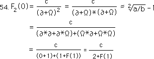
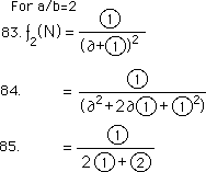
Let us now look at a more ‘normal’ situation, i.e. when the M of the general equation equals 2, i.e. the F series generates a square root. We substitute 2 for M in the general equation. We expand the equation in the normal way employing both the distributive and commutative properties to expand the equation and combine terms.
At the end of Equation 54 we obtain the same result for square roots that we derived before.
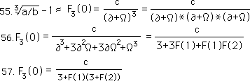
Following are the expansions of the cube and 4th roots. The patterns are made manifest. First the cube root series.
In equation 55, we start with the general equation and expand it. In equation 56 we substitute in the defined values for the powers of ∂ and Ω. In equation 57, we nest the values algebraically to give our F Series for the cube root its familiar form.
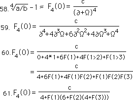
Now the expansion of the F Series for the 4th root.
First the general statement, #58, then the traditional binomial expansion, #59, followed by the substitution of the defined values, #60, and finally we show the traditional iterative function for 4th roots developed in this Notebook, #61.
What are some of the implications of this equation for the Binomialized F Series?
One gets the feeling that each additional root adds a layer of complexity, an actual dimension to the number in question. Normally multiplication implies adding dimensionality. For instance when mathematicians speak of the square or cube of some number, it refers immediately to its geometry. A number multiplied by itself twice yields a square, while a number multiplied by itself three times yields a cube. This same language is used in inverse for roots. The number that is the root of the square is called the square root, while the number that is the root of the cube is called the cube root. The root in this case is the one-dimensional line that when expanded into 2 or 3 dimensions yields the square or cube.
In the case above, while the first dimension is a line with magnitude, the ‘zeroth’ dimension is a point, which exists. Any number raised to the zero power equals one, while any number raised to the first power yields itself. Hence while a point has no magnitude, the line is shrunk from extension to just existence, which equals ‘one’ the identity factor for multiplication. These relations are shown below.
Now our ‘numbers’ are a little different. As Roots they would traditionally represent a line; a one-dimensional line. While it is easy to write Roots in this context, these Roots really have no real meaning except as an abstract concept. In this section we are trying to understand what Roots mean in terms of the general equation. It seems that Roots are really inverted dimensions. What this means, we have no idea. However while cubes and squares are generated in positive reality, cube roots and square roots are generated in negative reality. This is exhibited somewhat in the equation below by the negative exponent.
The root in this case is generated through the multiplication of the negative exponent. Thus to go from ‘normal’ one dimensional reality to the square root, one must ‘multiply’ normal reality by the next extension, i.e. by the extension into negative reality. Then to go from a square root to a cube root, one must extend into another dimension of negative reality.
Each of these negative internal dimensions is created by ‘multiplying’ the previous Root by the inverse of (∂+Ω), which we’ve seen is approaching ‘one’. Equation 53 is shown again below.
Thus it seems as if this ‘one’ established when ∂ and Ω are ‘added’ together is some type of inverted negative dimension which is added on to the previous dimension, just as in the positive realm each additional factor that is multiplied on to the previous raises the power and dimension by one. It is very similar except reversed. This is why we are calling it an extension into negative reality.
Further these extensions have to do with adding another layer of feedback. While in the positive dimension, there are no layers of feedback; a number is what it is. However in these negative or inverted dimensions each Root except the first are generated iterative functions. The square root only needs the past fed back in to generate its approximation, while the cube root needs the past two members of the series, and the fourth the past three members of the series to generate the next. Thus while ordinary reality is generated by adding dimension to dimension, our inverted reality is generated by adding another layer of feedback. These are self-reflective dynamic functions, very different from our ‘ordinary’ functions but similar at the same time. We are slowly going mad. Come on along. It’s fun.
Let us look at our General F Series from another perspective. First remember that our constant, c, is equal to our rational number minus one. Instead of a rational number, let us call it the real, or perhaps even the complex number, L. Restating our mission we are trying to find the Root of L, some complex number.
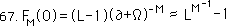
Substituting ‘L-1’ for ‘c’ in equation 64 we come up with the following formula.
We must remember that the left hand side of the equation is just the binomial expression of the General F Series, which approximates the Mth Root of L, minus one, expressed above. The Mth Root of L is expressed as L to the M to the -1 power, in other words L to the 1/M power, or the Mth Root of L. As the number of trials or iterations approaches infinity, the F Series value approaches this same Root. This is expressed below.
Our F Series has the peculiarity of being able to express every Root in the universe with its iterative series except zero. The only way our F Series equals zero is if L is equal to 1, in which case there is no series regardless of the Root. Zero is the only exact number in this iterative universe, all else are approximations.
This is a parallel with Data collection. Every piece of Data that exists, except unitary data, of course, is imprecise by virtue of the measuring standards and stick. The only piece of Data that is exact is Data that doesn't exist. If something happens, we can only approximate its Duration. While if something doesn't happen we can say that it exactly equals zero. On the most basic level of Data Collection, we can say that something happens or doesn't happen. However as soon as we get into Duration we simultaneously enter the world of Approximation.
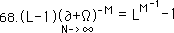
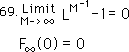
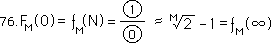
As M, the number of roots, approaches infinity, our F Series also approaches zero. As M approaches infinity, the inverse of M, i.e. L's exponent, approaches zero. As L's exponent approaches zero L1/M approaches 1. This neutralizes the '-1' in the expression for F(0). Thus as M -> ∞, ƒ(∞) -> 0. These relations are expressed below.
Restating our results: the Limit of our F Series approaches zero as M approaches infinity. Thus we can get as close to zero as we want by increasing the number, M, of the Roots, but our Root will never equal zero. When the mythical infinite iteration of the infinite root of any number is reached is when the F Series equals zero. Metaphorically zero exists as the Void, nothingness, or as the most complex level of iterative reality which is only an approximation. The ultimate complexity only approximates the spontaneous Reality of the Void.
We can also see from the above expression that we can’t find the zeroth Root. M is the denominator in the exponent and so can’t equal zero.
Thus our Fractional F Series expresses the whole universe of numbers as approximations. The only element in the whole F Series universe that is exact and precise is zero. This is what the Buddhists have said all along. The phenomenal world expressed by all of our Roots is simply illusion. We can imagine the precision, but it doesn’t really exist. The only thing that is real is the void, emptiness, Zero, the center of our universe, the point of origin, the Black Hole from which spews the imprecise illusionary phenomenal world in all of its fractal glory, striving impossibly after precision. We want laws, precise, always and forever correct, something that we can lean on. Instead we get these infernal approximations. We steadily approach alignment with the Tao but never really get there.
Now that we’ve examined the Binomialized F Series, let us binomialize the Denominator Series. The D Series has been with us for a long time, we can’t leave her behind now.
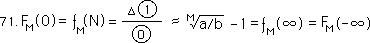
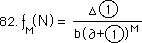
Let us begin by restating some of the generalized facts that we have discovered about the D Series. The first expression below shows how the F Series is a simple function of the D Series and how they both connect up to the Generalized Root. Remember ∆ = a-b. (Of course ∆ has the more general representation, expressed above in pervious sections, if we are speaking about fractional roots.)
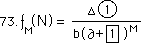
Below is the general derived expression for the Denominator Series, which is at the foundation of the F Series. The coefficients are supplied by Pascal’s triangle, as we shall see. (Again if we are speaking about fractional roots b would be raised to a power as would ∆.)
Binomializing Equation 71 with equation 72 for the denominator, we end up with following result.
We see our old friend the infinitesimal, something yet
nothing. You old, ambiguous, paradoxical thing – as the foundation of all
Roots you tickle my mind. Again it has the same definition. when operating, *,
on itself, no matter how many times, it always equals nothing. However when it
operates on the one square,  , it
always leaves it alone, like an identity operator. Of course the commutative
and associative properties apply because that is how the binomial expansion works.
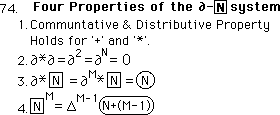
Below are the four properties of this ∂-
, it
always leaves it alone, like an identity operator. Of course the commutative
and associative properties apply because that is how the binomial expansion works.
Below are the four properties of this ∂- system
Although the first three are similar to the properties of the ∂Ω system developed with the F Series, the fourth property is significantly different. It has a significant multiplier, which the ∂Ω system didn’t have. Although raising Ω to the higher roots resulted in more multipliers, raising our square to higher levels just sends it more into the past. Thus the higher the Root the further one must reach into the past to arrive at the proper solution.
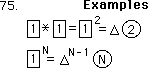
Below are a few examples of this type of binomial operation.
The multiplier adds a layer of complexity not found in the ∂Ω system, but there only two factors, while with the ∂Ω system there was one less unique factor than the number of the power. Each has its advantages as we shall see.
Now that we’ve seen the way that ∂ and  interact, let us examine some examples of
the D Series binomial expansion. Let us begin with the simplest of expressions,
i.e. when the Root Number is two.
interact, let us examine some examples of
the D Series binomial expansion. Let us begin with the simplest of expressions,
i.e. when the Root Number is two.
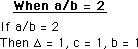
When our Root Number is two, all the extra multipliers, i.e. ‘c’, ‘b’, and ‘∆’, are equal to 1. These multipliers are sprinkled throughout both the Fraction and Denominator equations. When these constants are ‘one’ they simplify computation tremendously.
Let us look at our general Root Formula for the F Series when the Root Number, a/b, equals two. One gets the following beautiful result.
Let me say it in words. First, no matter which Root of two is sought, i.e. square, cube, or 25th, the formula is the same. Second, as the number of iterations increases, the simple ratio of the consecutive members of the appropriate Denominator series always approaches our Root minus one.
The equation for the appropriate Denominator Series is shown below.
The coefficients are given by the binomial expansion. Of course for simplification we could write the D Series in its binomialized form. This is what we get.
Remember that this is the special case when our Number is two.
Note that we’ve substituted the circle notation for the square notation. Originally we differentiated the two to make sure that the standard operation of multiplication was not confused with the operation, ‘*’, used in our binomial expansion with ∂. However we will use the circle notation here to emphasize the basic correlation between circle N and square N. The operation is different, not the elements.
Now we can write the general equation in binomialized circle notation.
The properties for our binomial expansion are the same as before. 1. The commutative and distributive properties both hold, allowing for the coefficients of the expansion. 2. ∂ when operating on itself always equals zero. 3. ∂ when operating on our circles always leaves them unchanged.
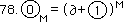
The only property that is changed is the fourth. When our circles operate upon themselves they just bump themselves into the past. There is no delta, ∆, coefficient. This revised property is shown below. (Let us emphasize that this equation only holds when the Root Number is 2.)
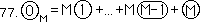
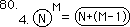
Following are a few examples of this type of operation. When circle1 operates upon itself once the result is circle2. When circle1 operates upon itself ‘N’ times the result is circle N.
To understand the context of this discussion, let us remember that circle0 is the Present Denominator of our series; circle1 refers to the Past Denominator; and the circle2 refers to two denominators before the present. Circle N refers to N denominators before the present. Hence each time a denominator is operated upon, it sends itself one more into the past.
Instead of trying to understand what this verbiage means, let us look at a few simple examples of the binomial expansion of our D Series. First we rewrite equation 73 in the circle notation mentioned above.
Let us look at the simplest expression for this General Root Equation. This is when our Root, M, is 2 and our rational number, a/b, also equals 2.
We notice that all the ∂ terms drop out, as if adding zero. We also notice that raising our circles to powers throws them further into the past. Step 85 is our well-studied Denominator Series for the square root of 2, developed in the previous Notebook.
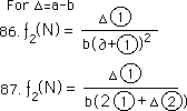
Similarly the General Equation for the Square Root of any rational number, a/b, is shown expanded from the general equation below.
Notice the appearance of ∆, which equals a-b, in the denominator of our expression. It is this term that creates the disturbances in our Bogus equations – to be discussed in the next Notebook.
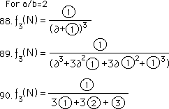
Now let us look at the expression for the Cube Root of 2. Remember when our Root Number is 2 that all of the relevant constants become equal to a 1 multiplier.
We arrive at an equation written only in terms of relative D Series expressions and the binomial coefficients; the same that we derived earlier.
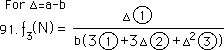
Now look at the general expression for the Cube Root of any rational number, a/b.
Notice the growing exponents of the delta, ∆, terms. It is these terms that both hold the True equation together and throw off the Bogus Equations under extreme conditions.
We now have all the equations with their unique properties to state our three basic Iterative Theorems in their most general expression. These three theorems allow us to generate any positive rational root solely through iteration. These are sometimes referred to as the General Root Theorems or as the Binomialized F&D Series for all roots. They are the foundation of our higher family of numbers.
The First Theorem for the F Series is stated in its most general expression below.
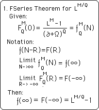
This is the F Series Theorem for all positive rational roots. L, M and Q are all constants. M and Q are positive integers while L is a positive rational number. Both N and R are also integers, representing the number of iterations. We state our theorem in both ‘small f’ and ‘cap F’ notational systems, which is defined here. Our binomial expansion of ∂ and Ω is delineated by the four properties listed earlier.
Below is our Second Theorem, the Numerator Theorem.
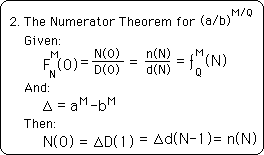
Again its expression is very simple. The N Series is a simple function of the D Series, to be delineated in the next theorem. Again we use both the ‘cap N and D’ and ‘small n and d’ systems to illustrate their essential equality.
Below is the Third Theorem, the Denominator Theorem for all rational roots.
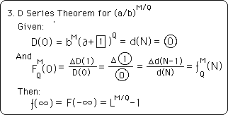
The ‘Given:’ defines our D Series expansion. The binomial
expansion of ∂ and  is determined by the
properties listed previously. Note that we express this relation in the Circle
notational system as well as the ‘small d’ and ‘cap D’ system to illustrate their
equivalence. The second ‘Given:’ defines the relation of the D Series to the F
Series. Again we use all three notational systems. The ∆ term is the same that
is defined in Theorem 2. The result is the same as Theorem 1. This just
affirms that this is the same F Series that was identified there although it is
generated in a different way, with different patterns.
is determined by the
properties listed previously. Note that we express this relation in the Circle
notational system as well as the ‘small d’ and ‘cap D’ system to illustrate their
equivalence. The second ‘Given:’ defines the relation of the D Series to the F
Series. Again we use all three notational systems. The ∆ term is the same that
is defined in Theorem 2. The result is the same as Theorem 1. This just
affirms that this is the same F Series that was identified there although it is
generated in a different way, with different patterns.