Home Science Page Data Stream Momentum Directionals Root Beings The Experiment
In the last part of this book we will explore a few related areas of mathematics; tie up a few loose ends; reach some dead-ends; and include some research upon π. Because of this hodgepodge of topics we call this Notebook Leftovers. The following topics will be dealt with herein:
1. First we extend the research of our square root paper looking at the Inverse Function of our Root Equations. 2. In searching for the slope of the Line of the Higher Roots, we reach some Dead Ends, which are exhibited and commented upon here. 3. Then we explore parallels between the Mandelbrot set and our Root Beings. 4. This exploration leads to an examination of the In-between Fractional Root and its significance. 5. This leads us into the unique properties of the Binomial Root System developed in these pages. 6. Finally we connect π and other ‘patterned’ transcendentals with the infinite continued fraction system. If the Reader has any curiosity left, read on. It’s worth it.
In Part I, Square Root Family, we succeeded in finding an ‘ordinary’ equation that would emulate our iterative expression for square roots. Intoxicated with success, we now delve into the higher roots. We remember from Part III, Root Beings, that the Difference Series for the Higher Roots is logarithmically linear in a similar way to the Difference Series for Square Roots. We would love to find the slope of these lines and we would love to write another complex equation to describe them.
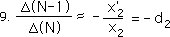
Let us see how we discovered the slope, i.e. the divine ratio, for our square Root Series.
This is the relation that we are trying to discover. It is the ratio between consecutive members of the Difference Series for square roots.
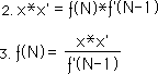
In our Notebook on the F& D Series for Square Roots we proved step 2. We called it the 7th Theorem.
Simple algebra transforms it into step 3. We substitute this expression for ƒ(N) back into equation 1 to arrive at step 4.
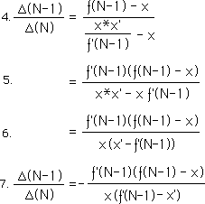
Some simple algebra yields the next steps. In step 5 we multiply the top and bottom of the equation by ƒ’(N-1). In step 6 we factor an ‘x’ out of the denominator. In step 7 we factor a ‘-1’ out of the denominator.
To move forward we need to introduce an intermediate theorem. We already proved the following two relations in the past Notebook.
First we subtract the two equations from each other.
This yields the intriguing result of equation 4. In words it states that the difference between the F Series and its limit, x, equals the difference between the inverse series, ƒ’(N) and its limit, x’.
We substitute this result into equation 7 above. The two factors on the right equal each other and therefore cancel each other out, equaling one. This yields step 8 below.
From the Square Root Notebook, we know that the limit of the inverse Series, ƒ’ is x’. We substitute this below.
Thus as the number of iterations, N, approaches infinity, the ratio between consecutive members of the difference series for square roots approaches the negative divine ratio, -d2. Bingo. That’s it.
This is the proof that we need to emulate to find the slope, i.e. the divine ratio, for the higher roots. We notice two elements that exist in this proof that we don’t have so far: the inverse series, ƒ’, and its limit, x’. Thinking simplistically, as always, we assume that if we can only find the inverse root and its limit that the Slope for our Higher Root Beings will immediately fall out from there. Then our complex spiral will emerge quickly from there. Therefore this section focuses upon the search for the inverse function and its limit for the higher roots.
Our General Root Formula consists of a single iterative fraction. The numerator, a constant, is a real number and the answer, the Root minus one is also real. Both of these are ‘normal’ numbers. However, combined with these ‘normal’ algebraic expressions is a weird denominator. It is the sum of an infinitesimal and generator raised to the N power. It creates the iterative expression. This section is going to focus upon that weird denominator.
What’s weird about it. It represents an iterative process rather than a static state. As opposed to ‘normal’ functions, one cannot speak specifically about what this iterative process equals. One can speak about what it equals after a specific amount of iterations. One can also say that the iterative function approaches or doesn’t approach a certain value. For instance it is proper to say: “What is the value of our function after 20 iterations?” or “What value does the function approach?” or “Does it approach a Limit?” It is improper to say: “What does the function equal?” Our iterative functions are always in process. While they may approach a destination incredibly rapidly, they never reach it. Indeed as we showed in a previous paper, the approach to this mythical Limit by the iterative functions that we are studying is actually erratically linear on a logarithmic scale. Hence from a logarithmic perspective their approach is quite steady and regular.
Another weird aspect to these iterative functions is that they cannot be treated with standard algebraic procedures. Because they feed upon themselves, i.e. past results, the pattern of regeneration is everything. Because this Pattern is so dominant in the process, anything that changes the Pattern changes the subsequent results in strange and seemingly unpredictable ways. One word that has been applied to dynamical functions is counter-intuitive.
We will explore some counter-intuitive properties of our iterative system later on. But for now let us examine an easy example on the most elementary level of one layer of feedback. Suppose our iterative equation is X1 = X02. If X is a positive number less than one, 1>X0>0, then the limit of our iteration is zero, X(∞) = 0. However if a simple one is added to the same expression, X1 = X02+1, the iterative result goes to infinity, X(∞) = ∞. Thus a simple one could easily drive the orbit from finite to infinite when added to an iterated function. The simplest operation of addition because of continual feedback can drastically change the results. The point here is only that the weird denominator turns the expression into an iterative function. Let us look a little more closely at this weird element.
Before our next exploration let us look at a few of the Theorems that we have proved.
This is our famous iterated Infinite Continued Fraction Series, which we mentioned above with its ‘weird’ denominator. The information is found in the F Series Theorem, Theorem 1, found in Higher Roots.
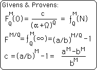
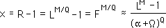
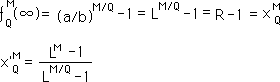
Let us return once again to the derivation of this F Series. We begin with the Given that L is any positive rational number, a/b. We call L the Root Number. We then Let X+1 equal the Root Number, L raised to the rational power, M/N. M & N, a & b are all positive integers. We call M/N the Power. The Root Number raised to the Power is called the Root, which we call R.
In a previous paper we derived a well-tested General Root Formula. This is shown below.
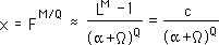
Our Formula is written in terms of X, which equals the General Root, R, minus one. The F Series is an iterative series based upon infinite continued fractions with the Root minus one as its limit. As the number of iterations approaches infinity, the limit of the series is X. The iterative expression is shown in its simplified binomialized form on the right. The approximation sign, ≈, in this case and throughout our Notebooks, indicates that after a finite number of iterations the answer is only approximate, while after an infinite number of iterations the result is exact.
Below is another equivalent representation with the constant, c, replacing the numerator. This is the constant we have used for simplification in other parts of our exploration. F raised to the Power is the limit of the iterative series. Remember the finite iterative series is only an approximation of X.
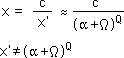
Now let us create an X’, which equals c/X.
We see that X’ equals a fraction. We know that X’ is a real number because c, the numerator of the fraction, is a constant, which is a real number, and that X, the denominator, is a positive root plus one, which is also a real number. Therefore X’ has a real value which can be computed and we will.
This creates the following interesting relations.
The first states that the limit of the F Series, which equals X, is also equal to c, our constant, divided by X’. Also the product of X and X’ is c.
Although this relation follows immediately from the definition, we will grace it with a theorem for ease of reference. This is the fifth iterative theorem, derived in the Square Root Family Notebook, Part I.
Lest we get carried away with parallels, and jump to some unjustified conclusions, let us note that although X’ holds an identical position to the Root Generator in the following equation, that they are not equal.
The Root Generator only exists as part of the whole iterative expression. It is not separate from it. If the Root Generator could become something it would become X’. But it doesn’t exist separately. While the musical notes make the music, one can’t isolate out the notes and find the music. Thus our Root Generator is the music, while X’ is its endnote. While X’ is the end limit it is not the music.
To illustrate some of the problems of equivalency, let us look at the following simple example, when Q =2. Expanding the Root Generator in the normal way we come up with the following expression:
F(0) = 2 + F(1)
In the previous treatments of this simple expression, i.e. when it was in the denominator, it didn’t matter what the seed was, because the series would always produce the appropriate square root. However in this example it is easily apparent that if the right hand side is treated as an independent iterative expression equal to F(0) that it will quickly move to infinity with any seed greater than -1. In no way or under any circumstance will it approach the value of X’, which we proved in the square root paper equals the Root plus one
Thus while X’ seems to equal the Root Generator or at least its Limit, in reality it only equals what the Root Generator could equal if it could have a separate limit, which it can’t.
Let us see what X’ equals.
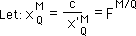
First we need some notational clarifications. In order to differentiate the order of the Xs and X’s we will use the same subscript, superscript method that we used with the F Series. It is assumed that each of these expressions has the same Root Number, L. The different Powers have different X and X’ expressions which we will explore.
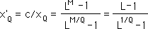
To further simplify matters and see where we’ve been, let us assume that M=1 in the following explorations. Then this is the notational shortcut that we will use.
Notice as is normal with ones, they disappear.
Let derive a usable expression to determine the value of X’. Following are the definitional extensions of X’ when we are finding simple roots, i.e. when M =1.
Following is the simple theorem, for easy reference.
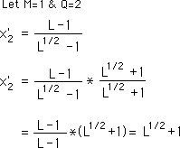
First let us look at the X’ for square roots and we discover an old friend. Employing the above theorem, we derive the expression for X’ for square roots that we derived in the earlier paper, i.e. the square root of the Root Number plus one, that we mentioned earlier.
Remembering that X equals the Root minus one, we multiply X and X’ together to arrive at L-1, which equals c, confirming our algebra.
Let us tackle something a little more difficult, X’ for fourth roots. Remembering that X4 equals the fourth root of the Root Number minus one, we substitute in the Theorem 5.2 from above.
Using the same technique as for square roots, we multiply the denominator by its reciprocal, twice, in order to simplify the expression. The L-1 expression that appears in the denominator cancels the L-1 expression in the numerator, leaving us with an intriguing product.
We notice that X’ for fourth roots is a function of X’ for square roots. This is written below.
Or we could just expand the product in normal fashion and arrive at the following patterned result.
We could factor this expression in the following way to get an expression that is very similar to the expression for the Mandelbrot equation, as we shall see.
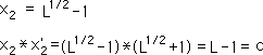
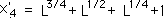
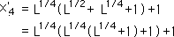
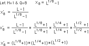
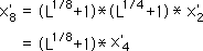
Now let us look at the X’ for 8th roots to expose the pattern for what it is.
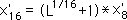
Using the same technique of reciprocals, we find the expression for X’ for 8th roots. We notice that within it are the expressions for the X’ for 2nd roots and X’ for 4th roots, shown below.
If we simply expand the product like we did before we get the similar intriguing result.
Using the same techniques we could also find the 16th root of X’. Shown below.
It is easily seen that it too is a function of the 8th root of X’.
The positive Root of any positive number is always positive. This positive added to one makes all of the multipliers greater than one. If they are greater than one then they expand a product. Because all the roots of X’ are all successive products of themselves, it would be easy to derive the following result.
Now let us look at the 3rd root of X’.
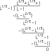
This is the same expression that we could so easily manipulate with reciprocals, before. However cube roots don’t break into reciprocals like multiples of 2. So we go with long division.
Amazing! It came out even. Thus along with the previously established pattern we arrive at this expression for the cube root of X’.
We can’t break this expression into a binomial expression like before, unless we invoke imaginary numbers, which don’t reveal any recognizable patterns. However we can turn it into a Mandelbrot type expression, like we did with the 4th root. This is shown below.
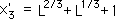
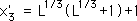
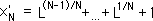
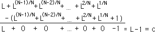
It is easy to generalize to the Nth root of X’. Basically we are looking for a reciprocal function, X’, that when multiplied times X yields L-1. Let us assume from our pattern so far that X’ takes the following form.
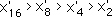
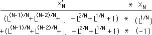
Now if we multiply X*X’ we should arrive at L-1=c. Let’s do it. X equals the Nth root of L minus one. This is the right hand column. The left column is the expression for X’.
If we multiply both parts of X times X’ and then add these parts together we will arrive at their product. This is shown below.
Multiplying the Root of L times X’ yields the top expression. Notice that 1/N is added to the exponent of each part of X’. Multiplying ‘-1’ times X’ only turns the addition sign on the left into a subtraction sign. Finally we subtract the top from the bottom and arrive at L-1, which equals c. Thus our educated guess for X’ was accurate.
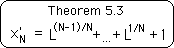
This is expressed in the theorem below.
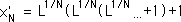
Factoring out as before we arrive at the following Mandelbrot type expression.
Thus once more we arrive at a nested version of these iterated equations. There are (N-1) L expressions and also (N-1) ‘+1’ expressions in the equation.
For comparison let us look briefly at the Mandelbrot nested equation, which we will develop in a following section.
We have the same series of constants in the beginning of the expression. In one case for the Mandelbrot equation the constant is c. While for the x’ equation the constant multiplier is the Nth root of L. Each of the expressions also end with a bunch of ‘+1)’s. The only difference worth noting, and an extremely crucial one, is that the ‘+1)’ expressions are all squared for the Mandelbrot equation while they are not for x’. Intriguing similarities with no connection.
Now that we have discovered what X’ equals let us look at the inverse Fraction Series.
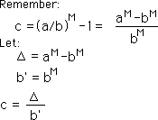
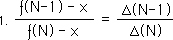
Let us remember the general expression for our constant ‘c’. Let us introduce a ∆ constant and a b’ constant for simplification. Then c simply equals the ratio between the two.
Let us now remember the general expression for the F series in terms of the Denominator Series, the D series.
We defined d(N) specifically in past Notebooks. It is not relevant to the present treatment. The ratio of consecutive members of this series treated as above yields the F Series.
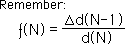
Let us now define an inverse series, ƒ’, based on the inversion of the fraction. The last member of the D series is now in the numerator while the preceding member is on the bottom. This is shown below.
If this were the definition for ƒ’(N) then ƒ’(N-1) would equal the following.
Multiplying ƒ(N) times ƒ’(N-1) would equal our good friend, the constant c. Shown below.
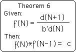
This is our next theorem.
We call it Theorem 6, as in the Square Root Theorems. Notice that it is identical except for the b’ = bM, which allows this expression to include all fractional roots. When M = 1 as in square roots, our inverse function is identical to the Square Root Theorem #6.
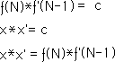
Combining Theorem 6 and Theorem 5 we arrive at the next theorem.
Since both the reciprocal product of finite series and infinite series both equal c, they obviously equal each other.
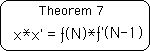
This is Theorem 7. It is identical to Theorem 7 for square roots.
Remember that this is for all fractional dimensions, not just square roots or cube roots.
Dividing both sides of Theorem 7 by ƒ(N) we get the top equation. We know that the limit as N approaches infinity of ƒ(N) is x. Therefore as N approaches infinity in the first equation, X/ƒ(N) approaches one. This leaves us with the third equation.
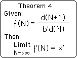
The inverse function approaches X’ as N, the number of iterations, approaches infinity. This is shown below in Theorem 4. Again it is identical to Theorem 4 for square roots.
Although we have left the superscripts and subscripts out for economy of statement, remember again that these formulas apply to all fractional Roots. These relations are reiterated below with their complete superscripts and subscripts.
This section has established the universality of the Inverse F Series Theorems for all rational roots. The Inverse F Series Theorems numbered 4 through 7 hold for all rational roots, not just square roots. Through these theorems the inverse F Series is defined in terms of the D Series. While the F Series is a ratio of consecutive members of the D Series, the inverse F Series is the inverted ratio of consecutive members. Both the F Series and Inverse F Series have limits. The product of these limits is our constant c. Further the product of specified finite members of both series also equals the same c. The finite product equals the product of the infinite Limits. Thus our System revolves around these polarities of finite and infinite, right-side-up and inverted. These polarities are contained in the Inverse Series Theorems.
Well now that we’ve achieved our goals of determining the inverse F Series with its Limit, we can now move on to the glory of finding the Slope of the Line for Higher Roots by using the same techniques we did when we discovered the Slope for the Square Root Line. Will it work? We don’t know. You must read on into the next section to find out.