Home Science Page Data Stream Momentum Directionals Root Beings The Experiment
Much of the previous exploration was based upon the desire to find the slopes of our Root Beings. How fast do they approach their limit? We wanted to generate another neat little expression that would express the general slope just as we generated a general inverse function and limit. Well let us see what goes wrong in this search for simplicity.
Let us begin with the good news, the experimental news. Let us begin by analyzing a table containing statistical correlations and slopes for the 3rd and 4th roots, as we did for the square roots. This should tell us enough to justify an investigation.
The title of the Table is ‘Correlations & Slopes for Log of Difference Series for 3rd & 4th Roots’. In the upper left hand corner is a box which contains, Num3/Den3 = 200/1. Those are the variable names that we use in our iterative functions. The number Num3/Den3, is the Root Number for this table. It can be changed to any decimal number to get similar results. We have just taken a ‘snapshot’ of the chart when this Root Number happens to be 200.
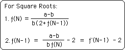
Below the root number are 7 columns, which are grouped into three sections. The first of these sections is the first column, which has to do with the number of iterations. The second three columns have to do with the cube root, while the final three columns have to do with the fourth root. The second column is the F Series for cube roots generated with the iterative equation for ƒ(N) listed at the bottom of the page. Column 3 is the Difference Series, which equals the difference between the F Series and the Root minus one. This column tracks how quickly our F Series for cube roots approaches its Destiny. The fourth column is the logarithm of the absolute value of the 3rd column. The next three columns are a duplicate of the past three columns, except that they pertain to the 4th root rather than the 3rd root. The fifth is the F Series for 4th roots for the Root Number that is in the box on the upper left. The F Series for 4th Roots is listed in the box at the bottom right with the F(0) notation, which we’ve used throughout interchangeably with the ƒ(N) notation. The 6th is the Difference Series and the 7th is the log of the Difference Series, as before.
Below the 100 iterations in the first column are two rows labeled ‘Correlation =‘ and ‘Slope =‘. These refer to the correlations and slope of the best-fit line between the next 6 columns and the first column, i.e. N, the number of iterations. The first two columns of the cube root have identical correlations and slopes as do the first two columns in the fourth root section. This is to be expected because the Difference Series is only a constant difference from the F Series. The correlations are weak, only about 17% each for cube and fourth root. This correlation is probably based upon how quickly this column approaches the exact root from an ordinary perspective, judging by the flatness of the slope. In both cases the slope of the best-fit line is under .04, i.e. 1/25. Looking at a graph it is obvious that this relation is in no way linear. We only showed the correlations to show how remarkable the next correlation is.
The correlations of the Log column of the cube and fourth roots show an incredibly strong linear relation at over 99% for both, nearly 100% correlation. The slopes for both are negative, as expected. The F Series for the Cube Root moves more slowly to its destiny than the F Series for the 4th Root, as expected, at 0.12 and 0.15 respectively. These results were seen in the Roots Beings Notebook. The higher the Root the quicker the approach. Therefore these logarithmic lines have a distinct slope.
Below the slope of the best-fit line are some theoretical slopes, which don’t fit. The rest of this section has to do with this dead-end. Don’t read on unless you’re curious about the results of failure.
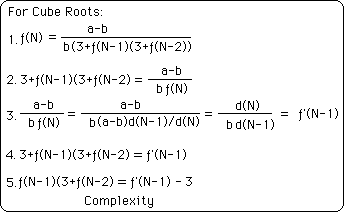
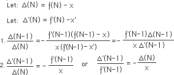
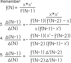
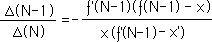
Let us remember or look back at the slope proof for square roots that we duplicated above. Steps 1 through 7 apply universally for all roots, because of the universal fact that ƒ’(N-1)*ƒ(N) = x * x’ = c is true for all roots, not just square roots. Below is the intermediate result that is universal for all Roots.
We are only a few steps from the end. This is going to be easy. A nice universal solution for the slope of Root Beings is just around the corner, we assume.
Let us move on to the next part of the proof, the little intermediate theorem, that ƒ(N-1) - x= ƒ’(N-1) - x’. We proved it for the F Series for square roots. We used two other intermediate theorems to prove this. Let us start with the theorem expressed in step 2, x + 2 = x’ for square roots. We could also rephrase this as x’ - x = 2. This is the difference between x’ and x. In our treatment of the square root series this simple difference between X’ and X was crucial for the above slope proof. Let us examine this difference for the higher Roots.
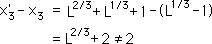
Let us look at a few of these differences beginning with the square roots.
The difference between x’ and x for square roots was simply 2. This amazing fact was the one that proved so helpful in the derivation of the Slope of the Root Being Line for square roots. Finding this slope revealed so much information about our F series that we called it the divine ratio.
Let us look at sampling of other differences between X’ and X.
For cube roots, the difference, while containing a 2 also has another weird element.
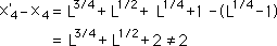
For fourth roots, the difference, while still containing a two, adds in two other complicating elements.
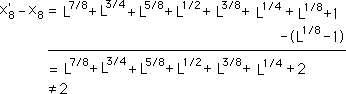
For eighth roots, the difference, while still containing a two, adds in many other complicating elements. The point is that while the difference between X’ and X for square roots was a simple 2, the rest have more complicated expressions.
Uh oh! This is a major glitch. While daunted, we will proceed forth to the other aspect of that small intermediate proof, hoping that something will drop out for clarifications sake.
The second little intermediate theorem that was used in our intermediate proof was ƒ’(N) - ƒ(N) = 2.
Below is the simple proof.
Now let us see how this simple proof manifests as the F Series of the cube roots.
In step 1 we use the iterative expression for cube roots instead of square roots. Notice that the expression has two layers of feedback instead of the one layer of feedback found in the square root expression. This is to prove fatal. In step 2 we switch numerators and denominators as we did above in the square root proof. Step 3 shows that the expression on the right in step 2 equals the inverse F Series, specifically ƒ’(N-1), as above. In step 4 we substitute this expression into the equation from step 2. In step 5 we find that we have a three, instead of a 2 to deal with. Further we have a (3+ƒ(N-2)) factor to deal with. This approach only leads to further complexity. This certainly doesn’t lead to any universal solution.
As a hint to the future, let us leave a few correspondences behind that might help solve the puzzle. And may be only a distraction.
We will only list the relations, seeing as how we couldn’t take them any further to solve the slope of the best fit line. Basically these relations relate inverse difference series and inverse F Series with the Difference series and their related F Series.
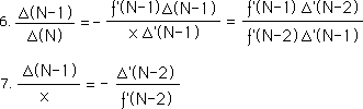
Basically these relations go around and around in circles, as step 7 is virtually the same as step 2.
Anyway, while yielding many fruitful relations between these factors, we could not isolate the slope no matter how many ways we tried. But this end might be a starting point for someone else. We at least tried to look over the fence. Someone else might have to stand on our shoulders to look over, however.
Let us finish off this section with one more dead-end. Remember the Universal Theorem for square roots, Theorem C. It stated that no matter which coefficients were used in a second order iterative equation based upon the sum of the two previous members that the ratio of consecutive items is related to a square root. Let us see if this Theorem can be extended to any of the Higher Roots.
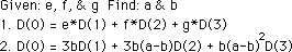
Let us begin with the cube root. Our problem is simply to find out what a and b are given the coefficients e, f, &g in the following expressions.
More generally put, the question is: Are all third order iterative equations based upon sums related to some cube root?
We base this proof on the equivalency of the coefficients in front of each of the iterations. This is similar to the equivalencies established in linear differential equations. Our first equivalency is that between the coefficients in front of the first iteration, D(1). We know that the coefficient of D(1) must equal 3b for the D Series for cube roots. We have already assigned this a value of e, which is given.
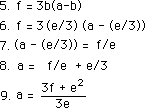
Therefore, using simple algebra b equals e/3, step 4.
In a similar fashion we set the coefficient of the second iterative term equal to each other, step 5.
First we substitute e/3 for b in equation 5, step 6. Solving for a, we divide by e, step 7, Then we add e/3 to both sides of the equation, step 8. Finally we combine fractions to arrive at an expression for a, step 9.
We have an expression for both a and b in terms of e and f. End of proof, right? No matter which values are set for e and f, we can always find some a and b that will satisfy the iterative equation. While this is true, there is one more coefficient to be dealt with, g. If the value of g has no influence upon the preceding events then the Universal Theorem will hold for cube roots. However, any condition that is placed upon its value limits its manifestations. Let’s see what happens.
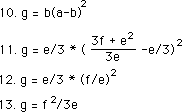
We start the same way as before, setting the coefficients of the third iterative term equal to each other, step 10. We then substitute the terms that we derived for a and b in steps 4 and 9 above, step 11.
We simplify the term inside the parenthesis, step 12. Multiplying through by e/3 we arrive at a simplified expression for g, step 13.
Let us look at the implications of equation 13. The terms a and b are determined by the first two coefficient e and f alone. Once these two terms are determined then g must equal the term from equation 13. It has no latitude beyond this relation. Thus while e and f can be any value to determine the values for a and b, the value of g is tightly proscribed. It must be the square of the second coefficient divided by the first coefficient times 3. Because the third coefficient is so constrained, the Universal Theorem does not hold for cube roots. Similarly it can be easily shown, in a similar fashion that with each successive root that specific constraints are placed upon each coefficient but the first two.
Let us demonstrate. For convenience let us call PN, the Nth coefficient of Pascal’s Triangle. P0 would equal 1 and then P1 would equal M the number of the root and so on. Further because of the symmetry of Pascal’s triangle the last coefficient PN would also equal one and the second to last coefficient PN-1 would equal M. This is shown below.
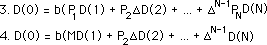
Now let us rewrite the general D Series expression with Pascal’s Coefficients. This is shown below.
Notice the use of Pascal’s coefficients in front of the successive D expressions, step 7. In step 8 we merely substitute the known values for P1 and PN. Now let us write the expression for a general Nth order iterative expression, with the constants e, f and g as coefficients.
If ‘e’ represents the first coefficient of the D Series then it will always equal P1*b or M*b, step 3. This means that b must always equal e/M, step 4.
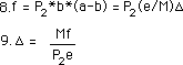
Similarly if ‘f’ represents the second coefficient of the D Series then it will always equal P2*b*(a-b). Remember that b = e/M and that ∆ = a-b, by definition. These concepts are shown in step 5.
In step 6 we merely solve for ∆.
Let us remember that in the general D Series equation that ‘a’ never appears separately. It always appears as an ‘a-b’ expression, which is signified by ∆. This is shown equation 1 and 2 above. This is why we don’t bother to solve for a.
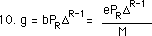
It is easy to conceptualize that if g represents the coefficient of any D expression except e and f that it will equal b times some Pascal’s coefficient of varying size, times ∆, as expressed in step 6, raised to some power, exactly. Shown below. The last expression just substitutes e/M for b.
Thus once two of the coefficients are determined then all the rest are automatically known. Although two coefficients have ultimate freedom of expression, none of the rest do. Thus we can write a Universal Theorem for a second order iterative expression, while none of the others are that free. Every iterative expression has two layers of freedom but no more.
This means that while there is an infinity of multiple order iterative equations based upon summation that lead to a specific root, that there are also an infinity of other coefficients that lead to an unknown Destiny, if at all. For instance the following D Series has no cube root associated with it, although it does approach a distinct Limit, shown through simple computer experimentation.
d(N) = 3*d(N-1) + 3*d(N-2) + 2*d(N-3)
The ratio of this D Series approaches a distinct but unnamable Limit. The Limit is not any rational root. Therefore it is a transcendental number. It is however generated by the pattern of the D Series. This the first example of a patterned transcendental, which we explore in more depth in our section on π.
The Universal Theorem does not hold for the D Series or for the F Series. In the F Series expression changing the coefficients of the denominator yield the same unnamable Limits as do the D Series. We saw this in the Notebook on Root Beings. We called these False Root Beings, because they didn’t approach the Limit under any Circumstance. Thus for every F&D Series which approaches a rational root limit, there are many other F&D Series which approach Limits which are not rational roots. Because there is a pattern that generates these number we call them patterned transcendentals.