Home Science Page Data Stream Momentum Directionals Root Beings The Experiment
In the last 2 sections we learned a little more about our System of iterative functions, which generates all rational roots. We learned that the True Root Beings of any level participate in the polarity of the F series and its inverse. This polarity connected the finite term and the infinite Limit in a simple formula. While we were able to achieve universality in terms of the F Series and its inverse, this universality did not extend to certain key formulas that were needed to generate the Slope of the Line of the Higher Roots. The simplicity of the square root polarity turned into complexity with even the cube roots. Yin-Yang polarity thinking is inevitably overwhelmed by the spontaneity of the multiplicity. In the next few sections we are going to explore the organization and properties of our Root Being System. We are going to use the famous Mandelbrot set as a vehicle for this exploration. In the exploration of some parallels between the Mandelbrot set and our Root Beings, we will come to a deeper understanding of the System and its implications. Lest anyone get too excited, these are only parallels, not actual connections. However because of the complexity of the Mandelbrot set, even a parallel is quite exciting.
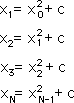
First let us look at what the Mandelbrot set is. This set is connected to an iterative equation, which we called the Julia equation in one of our previous Notebooks, where each new member is found by squaring the previous member and then adding a constant. This iterative equation is based upon one level of feedback and thus we call it a 1st order iterative equation. Following is the notation used by Professor Robert L. Devaney of Boston University in his educational video, The Fractal Geometry of the Mandelbrot Set.
The X0 that begins the sequence is referred to as the ‘seed’ of the iterative equation. ‘c’, represents a constant in the above equations, and can represent any complex number. The ‘orbit’ of the seed is the sequence of numbers that are generated by each successive iteration, i.e. X1, X2, X3, ... XN. For the Mandelbrot set, they set the seed, X0, at zero. The Mandelbrot set contains all c values for which the orbit of 0 does not go to infinity.
The following is the notation that we have been using in these notebooks, with X(0) acting as the seed.
These simple equations are context-based for they are based upon what went before. However because nothing is changed after the initial conditions are set, we could also write this iterative equation as a content based equation. This means we have to write this equation in terms of initial conditions only. We cannot write it in terms of past results if it is to be content based. Content-based equations only need the initial conditions to generate a result while context-based equations need the intermediate results. If all phenomenon could be broken into content-based equations as some scientists think then everything about the world has been predetermined. However if life responds to intermediate results then this reflects the mechanism of free will. Let us generate the content-based equation that would determine the ultimate orbit of our iterative equation.
Let us start at the simplest case. This is when our seed, X(0) = X0 = 0, equals zero.
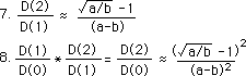
This would mean that X1 = c. This is shown below.
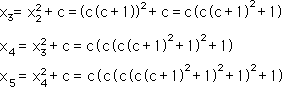
In the equation below for X2 we first use the above substitution for X1 . We then factor out a c. This gives us the rightward expression for X2.
We use this same process to generate X3, X4 , and X5, also. These are shown below.
Extending the same process indefinitely we easily arrive at the following expression for XN.
As a clarifying note on the above equation, there are as N 'c's and (N-1) '+1's. Further each of the parentheses is squared except the last one. Note that this content-based equation for the Mandelbrot set is quite complicated compared with the context based equation shown above.
However, as always, our content-based equation reveals a lot of information, which is not immediately apparent in the context based equation in the middle. For instance, the nested expressions are always squared. Therefore if the absolute value of ‘c+1’ is greater than 1 then the result quickly expands and the orbit moves towards infinity. Conversely if the absolute value of ‘c+1’ is less than 1 then the orbit moves towards zero. Therefore c must be between 0 and -2, not inclusive, for the value of c to be in the Mandelbrot set, i.e. its orbit doesn’t move towards infinity. Of course this only applies to the real number line, which is only a small part of the Mandelbrot set.
Now that we have explored the algebra of the Mandelbrot set, let us move on to its geometry, which it is famous for.
When the Mandelbrot set is graphed in the complex plane, it yields ‘one of the most beautiful objects in all mathematics’ according to Professor Devaney and disputed by few. For the purposes of this paper we will describe the Mandelbrot set as a central ‘bulb’ surrounded by an infinity of ‘bulbs’ of different sizes and shapes. Each of these bulbs represents a subset of complex numbers from the Mandelbrot set that have unique and identifiable properties, separating them from every other bulb. Each of these bulbs can be characterized by a unique fraction. The denominator of the fraction represents the period of the number within the bulb, while the numerator represents the method in which this period is manifested.
Let us be a little more specific. Every number that is not in the Mandelbrot set represents a c-term that drives the orbit of 0 to infinity. Every number in the Mandelbrot set represents a c-term that does not drive the orbit of 0 to infinity. All of the elements of the central bulb represent the c-terms that drive the orbit of 0 to a single point. All the elements of the large bulb on the left of the central bulb represent the c-terms, which drive the orbit of 0 to two alternating points. All the elements of the large bulb on the top of the central bulb represent the c-terms, which drive the orbit of 0 to three alternating points. All the elements of the large bulb on the bottom of the central bulb also represent the c-terms that drive the orbit of 0 to three alternating points. The top and bottom bulbs both have a period of 3. The members of each bulb have the same period as all the other members of the set. The period refers to how many different limits the members of each bulb have.
The main difference between the top and bottom bulbs which both have a period of 3 is that the top bulb hits its elements one after another in a counter-clockwise sequence, while the bottom bulb hits every other node in the same counter-clockwise sequence. Therefore the top bulb has a numerator of 1 while the bottom has a numerator of 2. Therefore the top bulb is characterized by the fraction 1/3, while the bottom bulb is characterized by the rational number 2/3. Thus the denominator refers to the period of the orbit of zero with these particular c-values, while the numerator refers to the way this period is manifested in a counter-clockwise direction. If the numerator is 4, it means that the period is manifested by every fourth element in the counterclockwise direction.
There is another way that we can describe this phenomenon geometrically. From the outside of each bulb a main root extends with a number of spokes coming off this main root from a central hub. The number of spokes emanating from this hub including the root is the period of the bulb. Counting counter-clockwise from the main root to the smallest spoke gives the numerator to the unique fraction that characterizes the bulb. This numerator, as explained above, reveals the way that the period manifests.
Reiterating, each bulb that surrounds the central bulb is characterized with a unique fraction. How are these bulbs organized around the central bulb? As mentioned above, the central bulb is characterized by the fraction 1/1, unity. The bulb on the top is given the fraction 1/3, the one on the left is 1/2, while the one on the bottom is 2/3. Between the large bulb on the top, 1/3, and the large bulb on the left, 1/2, is smaller bulb, characterized by 2/5. Between this bulb and the 1/3 bulb at the top is another smaller bulb, called the 3/8 bulb. Between the 2/5 bulb and the 1/2 bulb is another smaller bulb, characterized by 3/7. Between every two larger bulbs is a smaller bulb whose fraction is found by adding the numerators and denominators of the surrounding larger bulbs. In this way the border of the Mandelbrot set is formed.
From a distance the Mandelbrot set appears to have a central bulb surrounded by a few smaller bulbs. However as one moves in closer the edges of each of these bulbs appears fuzzy. This fuzziness is the infinity of smaller bulbs between the larger bulbs. If small sections of the border of these bulbs are magnified, they are seen to contain many smaller bulbs. No matter how many times a section is magnified more of these tiny bulbs emerge with all of their incredible order. While the borders appear to be fuzzily chaotic from a distance, on closer inspection they are incredibly organized.
Further these bulbs are organized as fractions on the real number line from smaller to larger going counter-clockwise around the central bulb. There is no bulb on the right. This is the zero bulb. Proceeding counter-clockwise around the border we eventually arrive at the 1/3 bulb on the top. Between this bulb and the zero bulb are an infinity of bulbs that represent every fraction between 0 and 1/3 in numerical order. Between the 1/3 bulb on the top and the 1/2 bulb on the left are an infinity of bulbs, which represent every fraction between 1/3 and 1/2 also in numerical order. Between the 1/2 bulb on the left and the 2/3 bulb on the bottom are an infinity of bulbs, which represent every fraction between 1/2 and 2/3 still in numerical order. Between the 2/3 bulb on the bottom and the 0 bulb on the right, (or 1/1 bulb in the center, same difference as we shall see) are an infinity of bulbs, which represent every fraction between 2/3 and 1/1 also in numerical order. Therefore the perimeter of the central bulb contains bulbs of different sizes, which represent every rational number between 0 and 1, in numerical order from smallest to largest in the counterclockwise direction.
Now that we’ve learned a little about the Mandelbrot set, let us examine a process, which we call The Process in the subsequent pages, which is the connection between the Mandelbrot set and the Root Beings. Let us look at the simple proof, which is foundational to the Process that numerically orders both the Mandelbrot set and our Root Beings.
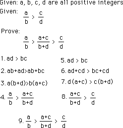
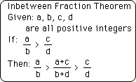
We begin with the knowledge that a/b is greater than c/d, where a/b and c/d are both positive fractions. These are givens. We then multiply both sides of the given by b * d to arrive at steps 1 and 5. We are solving the two conditions to be proved simultaneously because the technique is the same. In step 2 we add a*b to both sides of equation 1. In step 6 we add c*d to both sides of equation 5. In step 3 we factor an ‘a’ out of the left side and a ‘b’ out of the right side of equation 2. In step 7 we factor a ‘d’ out of the left side and a ‘c’ out of the right side of equation 6. In step 4 we divide both sides of equation 3 by b*(b+d). In step 8 we divide both sides of equation 7 by d*(b+d). We combine the results of steps 4 and 8, to arrive at step 9, which is the fact that we were attempting to prove.
This is the In-between Fraction Theorem. Shown below.
This proof establishes simply that adding the numerators and denominators of any two fractions creates a fraction that is between the two creating fractions in value. Thus, performing the process indefinitely, i.e. adding numerators and denominators to create an in-between fraction, creates a relatively solid mesh of fractions, infinite in size, between any pair of fractions. Repeated in a little different language: There is a chasm between any two fractions that is spanned, only partially, by an infinity of discrete fractions.
While the fractions themselves are relatively distinct, the limits of the process might be a fraction or it might be a square root. For instance in the rational category. We start with the two diametrical opposites, existence, the fraction 1/1 and non-existence, 0/1, which curiously enough start from the same non-existent point or limit. The point between, by our standard process of adding numerators and denominators, is the first polarity 1/2, the bulb whose c-values send the orbit of 0 bouncing back and forth between two values. Now if we consistently choose to always marry the new fraction with emptiness, 0/1, then the limit approaches but never reaches 0. It goes from 1/2, to 1/3, 1/4, … 1/N, …, 1/∞ = 0. Remember this a theoretical limit only. Similarly if we choose to consistently marry the new fraction with unity, 1/1, then the limit approaches but never reaches 1. It goes from 1/2 to 2/3, 3/4, 4/5, 5/6, … (N-1)/N, … (∞-1)/∞ = 1. Again this one is only theoretical limit, which doesn’t exist. Ironically because the central bulb is sort of round, encompassing all the fractions between 0 and 1, the origination point 0 and the end point 1 are one and the same point, both approached from different directions.
It is as if the path of spirituality and emptiness approaches the same point as the path of materialism and substantiality although from a totally different direction. In China we see this archetype with the Sage, the spiritual master, advising the Emperor, the material master. In a little different context we see the Pope balancing his spiritual power with purely political power of the kings and emperors of Europe. The Alchemical Taoists view this as the magic point when the Conscious Knowledge of the Emperor allows the Real Knowledge of the Spiritual Master to be made manifest. Similarly it is the miracle of the inner spiritual being manifesting through the gross material body. In all cases it is the miracle of manifestation from the merger of opposites. Remember also that neither exists without the other. While all moves after the initial move can be based purely upon emptiness 0/1 or substantiality 1/1, the initial union, which gave birth to polarity, 1/2, needed both emptiness and substantiality to manifest. Anyway these concepts are contained in the geometry of the Mandelbrot set.
Further the limit of any of these processes when the same partner is continually chosen in marriage is that partner, if it consistently chosen from the beginning. If even one different partner is chosen then the limit will be different, never to return to the original. However anywhere along the line if the partner remains consistent throughout the limit will be that one. Hence there are an infinite number of these paths whose limit is the fraction that is constantly remarrying with its offspring. This type of infinite reproduction always produces rational numbers as the offspring.
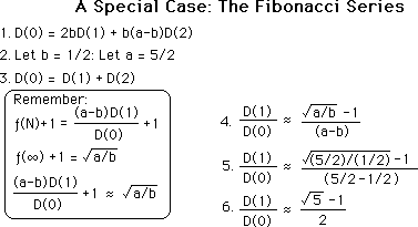
While the type of reproduction illustrated above always produces rational numbers, there are infinitely more types of this endless reproduction that yields non-rational numbers. One type, which we will examine now, yields square roots as its limit. The first that we will examine is based upon a familiar figure in mathematics, the Fibonacci sequence. In this case, instead of leaning on substantiality or emptiness, we instead marry for balance instead, always choosing to marry the union with the parent who has the largest denominator. In this case our series begins normally 0/1 + 1/1 = 1/2. (Remember that the addition sign signifies the marriage of two fractions, while the equal sign points to the union.) 1/2 + 1/1 = 2/3. 2/3 + 1/2 = 3/5. 3/5 + 2/3 = 5/8. 5/8 + 3/5 = 8/13, and so forth. We notice two things. First when choosing the largest denominator as the partner we continually alternate between larger and smaller instead of hugging to one side or the other of the fractional pattern. Second we see the same pattern that we established in the first Notebook of this series as the foundation of the denominator series, i.e. the new numerator equals the old numerator. Remember that this ratio leads to the distinct irrational number, (√5-1)/2, as outlined in the first notebook. Below is the short proof duplicated from the first Notebook.
Another square root limit is the smaller Fibonacci limit. Instead of continually choosing the largest denominator, choose the smaller in the first union and then the largest from then on. This is the sequence we arrive at. 0/1 + 1/1 = 1/2. 1/2 + 0/1 = 1/3. 1/3 + 1/2 = 2/5. 2/5 + 1/3 = 3/8. 3/8 + 2/5 = 5/13. 5/13 + 3/8 = 8/21. By paying attention we notice that the numerator, instead of being the past denominator, is instead two denominators past. Thus our fraction becomes XN-2/XN. What is its limit as N->∞?
Continuing our proof from above.
The ratio of any two consecutive members of the Denominator Series is approximately the same, i.e. approaches the same limit. Multiplying consecutive ratios by each other we arrive at the ratio squared, which is the limit of the ratio of every other member of the D Series to each other.
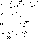
Thus it is now just a simple matter of plugging in our values for a and b, then computing.
Plugging in a = 5/2 and b = 1/2, we arrive at the above value for the smaller Fibonacci limit.
We demonstrated a well-known process for ordering fractions. This process was seen visually in the geometry of the Mandelbrot Set. The smaller bulbs surrounding the main bulb was each assigned a discrete fraction. Between any two larger bulbs was always a just smaller bulb whose fraction was determined by the Process. The Process repeated indefinitely proceeds to distinct limits. We showed both rational and irrational limits of the Process. Of course the most interesting rational limit was when the limit of something was nothing and vice versa. This paradox occurs at the same point in the Mandelbrot Set. Further two irrational limits were determined by variations of the Fibonacci Series as a Denominator Series. That’s all.
How does the Process, which orders the bulbs of the Mandelbrot set, connect with the Root Beings. We don’t know. You’ll have to read the next section to find out.