Home Science Page Data Stream Momentum Directionals Root Beings The Experiment
Now that we have successfully examined the Higher Roots from the F&D perspective, let us take a quick look at π and other transcendental numbers from the perspective of our new Family.
Let us first look at a micro-history of π.
π is the ratio between the circumference and the diameter of the circle. This great ratio, reflecting such a balanced order, has been approached from different standpoints throughout the ages. Each mathematician interprets it from the perspective of his age. Early on it was looked upon as a ratio. The Bible interpreted it the most simply as exactly a 1 to 3 ratio, of diameter to circumference of the circle. The Bible based religions always look for absolute truths. Within the same time frame, the Mesopotamians used the ratio of 22/7. In these days, there was no concept of mathematically exact. Instead the concept was of practicality. For the Mesopotamians, this ratio was close enough for practical purposes .
With the Greeks came the mathematically exact. Archimedes gave a more precise ratio. However the Greeks came to realize that certain numbers couldn't be expressed as an exact ratio. Thus Archimedes acknowledged that this was only an approximation. He gave two ratios that π must fall between.
This was the state of the art for some 2000 years. In the duration Archimedes' approximations were refined but not extended theoretically. With the renaissance of math and the sciences at the end of the Middle Ages, π was finally expressed exactly in an equation. Francois Viete (1540-1603) in the 1600s wrote the first precise rendition of π as an infinite square root series. From then until now, many other series have been written which express π exactly. This is his series. It will do nicely to indicate the fractal nature of π .
Here we are in the fractal 1990's. What is more appropriate than to explore the structure of π as a fractal. We are still going to write π as an infinite series, but we are going to explore its fractal elements. Even Archimedes realized that π would be realized in an infinite refinement but just didn't have the algebra to express it.
Before proceeding let us look at a popular infinite expression of π, which is not fractal and actually supplanted the early fractal representations. John Wallis (1616-1703) discovered a representation of π that became the most popular infinite representation of π because of its relative ease of representation and computation.
Although this representation has many other modern applications and derivations it is not a fractal representation. A fractal representation must reflect itself in the largest and smallest levels. It must be nested. Although this equation is exact it does not reflect itself upon any level.
Let us return to Viete’s representation of π. Let us treat it in the same way that we did the infinite continued fraction. Let us create a series of approximations whose limit is the infinite representation of π given by Viete. We have called these fractal function sets in other contexts, because each element of the series contains all the elements that went before. Each element of both our F&D Series’ contained every element that went before. Therefore we also called these fractal function sets. As we shall see they could also be called iterative functions because each member of the series is based upon that what went before. Every iterative function generates a fractal function set, because each new member contains all the members that went before.
For ease of visualization let us write Viete’s representation again.
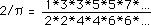
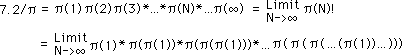
From this we can also write 2/π as the product of an infinite number of π functions.
Then π itself could be written as this infinite product.
What are these π functions?
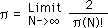
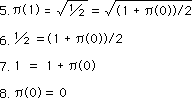
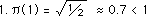
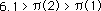
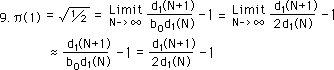
We begin with π(1), the first multiplier.
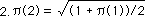
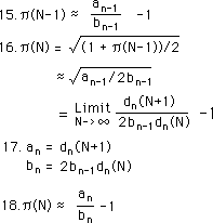
π(2) and π(3) can be written as functions of π(1) and π(2) respectively.
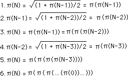
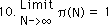
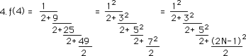
This leads us to a general expression for π(N).
Our π function series is self-referential. Each term is a function of the preceding term. This is a first order iterative equation. As mentioned self-referential series, i.e. one based upon an iterative function, always leads to the fractalization of its individual members.
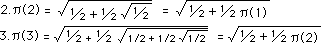
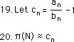
Further every first order iterative equation has one seed. What is the seed of our iterative π function? Starting with the expression from Step 4, we backtrack. From Step 1 we know what π(1) is. We also know that it is generated from the preceding term π(0), which is the ‘seed’.
Squaring both sides of the equation we get Step 6. Multiplying the equation by 2 we get Step 7. Subtracting one we get Step 8, which proves deductively that π(0) equals zero. Note that this specific ‘seed’ of the π function is different from the F&D Series, where the seed does not matter at all.
Another feature of self-referential functions is that they are nested. This nested feature creates fractalized reflections. Below is the algebraic nesting of π. π(N) is a function of π(N-1), which is a function of π(N-2), which is a function of π(N-3) and so on to π(2), which is a function of π(1), which equals the nesting of the seed π(0). Eventually π(N) can be written as a nested function of π(0). Hence the first is reflected in the last as well as all the intermediate π functions.
Thus each member of the iterative π series is based upon the multiple nesting of the seed, π(0), which equals zero. Thus from nothing comes something. Each nesting of zero is an iteration by the π function. The number, N, of each member of our set is the number of times our original number has been nested or the number of iterations of the ‘seed’.
The elements of ‘ordinary’ equations, i.e. zero order iterative functions, i.e. functions with no layers of feedback, are not based upon the previous members of the set. Therefore there is no nesting. Because there is no ‘nesting’ in ‘ordinary’ equations, the individual elements are not fractalized, i.e. created from each other.
Our π function is self referential and nested reflecting its fractal construction. All iterative equations have this same fractal component, because they are all based upon the continued ‘nesting’ of the ‘seed’. Nesting in this case refers to applying the iterative function to the ‘seed’. First order iterative equations only need one seed, which in the case of the π function was the square root of one half, √1/2.
Remember that 2/π equals the limit of the product of the π functions, not the limit of the π function, as we shall soon see. Each member of the fractal function set for π consists of nested π functions, i.e. π(N) = π(π(…π(π(0))…)). It is the product of these nested functions that is the limit we seek. The complexity of the expression is shown below.
Note that we start with π(1) instead of π(0). This is just to keep with our original expression. We could just as easily written it in terms of π(0). Remember that π(1) = π(π(0)). This simple substitution would yield a result of the same nature.
Remember that 2/π is the product of these π functions. Hence the above representation shows that the whole series is based upon the seed π(0) of the first member, π(1), which equals zero. This is the only given fact. The other given is the π function. No other information is needed to generate these approximations for π. Thus our iteration of nothing yields the quantities that when multiplied by each other yields our desired limit, 2/π.
Note that our expression for π is doubly fractal. Each member of the set is a fractal of the preceding elements while the π limit is the product of these fractals. This contrasts with the F&D Series, where the desired root is the Limit of the series, not the limit of the product of the members of the series. Obviously π is not an ordinary Root Number. It is transcendental.
We mentioned that 2/π is not the limit of our π function. What is its limit? Let's start at the beginning. π(1) < 1.
This is the expression for π(2).
The expression under the radical is the average of 1 and π(1). Because π(1) < 1, π(1) is the smaller of the two numbers being averaged.
Hence the average will be > π(1) but less than 1.
The square root of any positive number less than one is greater than the number but less than one because the square of any number less than one is less than the number. Hence the square root of our average would be greater than the average but still less than one.
Because the square root of the average is π(2), we know that π(2) is between 1 and π(1).
Following this pattern we can say that the average of any of the π functions with one will always be greater than the π function. The π functions will never be greater than one, for their self-referencing pattern begins below one and the pattern pushes it higher but never past one.
The square root of the average will be greater than the average but still less than one for the same reasons stated above in the particular case.
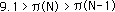
Because the root of the average is π(N), we can say that it is less than one while greater than π(N-1).
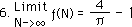
It is easy to see that as N->∞ that π(N) -> 1.
In another notation, π(∞) = 1. As before π(∞) means the limit of our π function as the number of iterations approaches infinity.
Let us look at our spreadsheet generation of an approximation for π. (See appendix.) Our series approaches the limit of the computer's 16-place precision rapidly. π(24) equals 1.00000000000000, 1.0 to 14 decimals, as far as the computer was concerned. The precision of this method rises rapidly. No more approach, our π series had reached its mythical destination. Similarly the value of computer's internal value for π is reached simultaneously with 2/π(24)!. Hence these practical limits are not out at π(1000), but instead surpassed the computer's computational abilities at only π(24). This is just a computer confirmation of the validity of our exploration.
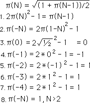
Just as we generated a negative D series for √2, here we generate a negative π series. We start with our general form of the series. We square both sides, multiply by 2, and subtract one from both sides of the equation. We then switch to the -N notation. We solve for π(0) as a function of π(1), which we already know has a value of √1/2. π(0) = 0. Similarly, using equation 2, we can solve for π(-1) = -1. The rest of the -π series all equal 1. If N > 2, then π(-N) = 1.
A mere curiosity.
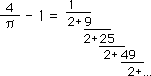
In decimal form π generates a non-repeating decimal. It is so irregular that it is sometimes used to generate random numbers. However in infinite continued fraction form, π becomes very regular just like the square roots. William Brouncker (1620?-1684) developed an infinite continued fraction for π. This is shown below.
We've already seen that all square roots can be written as an infinite continued fraction. These infinite continued fractions all have the same numerators and denominators. Hence the non-repeating decimals of the decimal notation become very rigid patterns in the infinite continued fraction notation. See below.
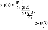
With this infinite continued fraction for π, we see that even transcendental numbers can be written as infinite continued fractions. But for π, our infinite continued fraction is still quite patterned. For each patterned transcendental, the numerator and denominator follows strict patterns. They are not fixed like the square root series, but still follow strict patterns. The numerators and denominators can be written as a clearly defined functions based upon the fractal function sets whose limit approaches the transcendental. Below is the derivation of the fractal function set for the patterned transcendental, π.
π is just one patterned transcendental. It is easy to see that there is a whole class of patterned transcendentals. The function (2N-1)^2 in the numerator of the π series could be replaced by an infinite number of precise functions, which precisely define an infinite number of patterned transcendentals. This is shown below with g representing any function, iterative or not.
In fact when this function is simply the constant, c, as defined previously, then the infinite continued fraction is the expression of a square root. This places square roots in the family of patterned transcendentals, which includes π. Square roots are simply a special case of the patterned transcendental when the g function is a constant
Each one of these patterned transcendentals can generate an infinite number of non-patterned transcendentals. At any point in the pattern an aberration can be introduced which will skew the result. The numerator or denominator at any point could be varied in an infinite number of ways, which would change the ultimate result. Thus for each transcendental there are an infinity of non-patterned transcendentals because for each fixed numerator or denominator there are an infinity of values that the numerator or denominator could have assumed. Hence for every patterned transcendental there are an infinite number of non-patterned transcendentals. Also a non-patterned transcendental can easily be generated by assigning random values to the numerators and denominators of our infinite continued fraction. Hence there are at least two classes of transcendentals, patterned and non-patterned. The patterned transcendentals include square roots, rational numbers and π, all in the same family.
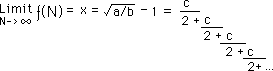
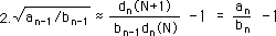
As a patterned transcendental, π is based upon the square roots of square roots of square roots ad infinitum. We've seen that square roots can be written simply as the limit of the ratio of consecutive members of the Denominator series. The defining equation is immediately below. (We used the inverse F Series representation instead of the F Series for economy only. The results are the same.)
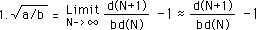
Hence theoretically π could be written as the limit of the ratio of the ratio of the ratio ad infinitum. What follows is an approximate suggestion of this reality.
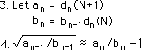
Above is the first equation written with subscripts in order to deal with a series of approximate ratios. The square root of the rational number, a/b, is approximated by one of the finite members of the D series, which can be the rational number whose square root is approximated by another finite member of another denominator series and so on. Equations 3 and 4 merely recognize this reality. The series of a's are the numerators of the finite members of the D series. The series of b's are the denominators of the same series. Equation 4 just restates Equation 2.
We serialize K and the D series also. Remember that the lower case 'n' represents the nth serialization of the D series while the upper case N's represents the Nth element of the series.
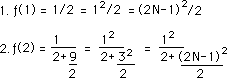
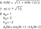
Now we are ready to explore. Equation 6 restates the general expression for the π function. Step 8 shows the initial elements of the a, b, and K series; and the expression for the first D series. These all follow from π(1) in Equation 7.
Using π(1) as an example of our series enumeration, we see the equality of the limit and the approximation of a finite member of this first D series to the square root. The initial members of the a and b series are constants, while all the rest are functions of the appropriate D series, which we shall soon see.
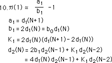
Step 10 illustrates the first elements of the a, b and K series, all results of the approximation for π(1). Also shown is the second D Series. It is a function of the first D series. It is easy to see that each successive series will be functions of the preceding series, which are functions of the preceding series etc. This is theoretical not practical.
Looking at π(2), we find a simplifying pattern. The number under the radical simplifies to our rational approximation divided by 2. Note that our specific b series is a simplification of the general b series specified above based upon the π function series. Equation 4 is a general representation, while equation 11 is the specific manifestation under the conditions set up. The second elements of the a and b series are shown. It is seen that they are functions of the finite members of the second D series. Finally we see π(2)'s approximation.
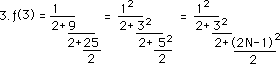
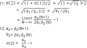
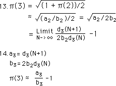
We apply the same process to π(3) and obtain parallel results.
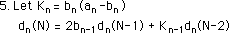
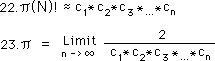
Generalizing our results we obtain an approximation for π(N). We also find the nth members of the a and b series.
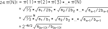
This approximation has a familiar term, a/b-1. We called this element, c, in the section on the polar nature of numbers because it was the product of the conjugate functions. Now because of its unexpected appearance in this unusual context, we introduce a serialization of c. This leads us to a greatly simplified expression for π(N)!. Appearances are deceiving. Each of the members of the c series are functions of the a and b series which are functions of the Denominator series, each of which is a function of the subsequent. Only theoretical.
We have one last expression for π(N)!. It is expressed here only because it simplified so easily. It is a pretty equation. But we have no idea what it might be used for. Aesthetics over function.
We looked at infinite continued fractions as a way of precisely expressing irrational numbers, including square roots and π. We realized these fractions were a way of including rationals and some irrationals, at least, in the same precise family. Belonging to this family led to the some interesting conclusions about numbers. Under this system, no number can ever be precise. A second aspect was that the underlying pattern used to generate the irrationals was more important than the data itself. The third aspect was the incredible crystalline structure. We examined the fractal nature of numbers, including patterned transcendentals, specifically the magical π.
The main topic of these many Notebooks has been Live Data Streams and measures that include decay, such as Decaying Averages, Directionals and Deviations. Although different formulas are used, it can be argued that the measures of the Live Data Streams are like non-patterned transcendentals while the measures of Dead Data Streams would be like patterned transcendentals. Hence our studies are examining the parameters of non-patterned transcendentals. Patterned transcendentals are exact in their requirements in the family of infinite continued fractions, although they are non-repeating non-ordered, chaotic decimals. Thus this Notebook places our Data Stream measures in a context.